Beyond the Scalar Friis Equation

Most communication system analyses rely on the simplified scalar form of the Friis transmission equation and often assume that many of its parameters remain constant:$$P_r = P_t \cdot G_t \cdot G_r \cdot \left(\frac{\lambda}{4\pi R}\right)^2$$

While useful for idealized scenarios, this form only represents a single operating condition, perfect alignment, perfect polarization matching, and a lossless free-space channel.

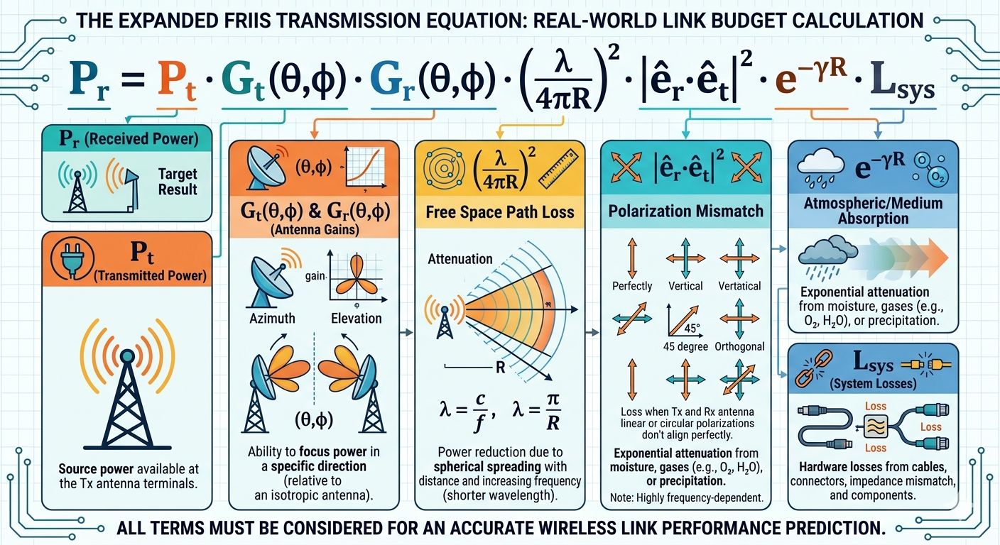
The more complete representation is the vector form:$$P_r = P_t \cdot G_t(\theta_t,\phi_t) \cdot G_r(\theta_r,\phi_r) \cdot \left(\frac{\lambda}{4\pi R}\right)^2 \cdot |\hat{e}_r(\theta_r,\phi_r) \cdot \hat{e}_t(\theta_t,\phi_t)|^2 \cdot e^{-\gamma R} \cdot L_{sys}$$

This formulation captures how real communication links behave under practical operating conditions.

Transmit Power $P_t$Pt​

Transmit power defines the total available energy budget. Every other term determines how much of that power successfully reaches the receiver. Doubling the transmit power results in a 3 dB increase in received power.

Transmit Gain $G_t(\theta_t, \phi_t)$Gt​(θt​,ϕt​)

Transmit antenna gain is not a fixed value—it depends on direction. Maximum gain occurs at boresight, where the antenna is perfectly aligned with the target. As the pointing angle shifts, the gain decreases according to the antenna radiation pattern, often following sinc² or Bessel² behavior depending on aperture geometry.

For example, a 0.6 m dish operating at 15 GHz with a beamwidth of approximately 1.8° may lose around 3 dB with a 1° pointing error. A larger 1.2 m dish with a narrower beam may experience a 9 dB loss under the same misalignment. Higher gain always comes with stricter pointing requirements.

Receive Gain $G_r(\theta_r, \phi_r)$Gr​(θr​,ϕr​)

The receive antenna behaves similarly. If the incoming signal arrives off-axis due to vibration, structural movement, wind loading, or thermal drift, receive gain also degrades. Both transmit and receive gains must therefore be evaluated based on actual operating geometry rather than ideal specification values.

Free-Space Spreading Term

$$\left(\frac{\lambda}{4\pi R}\right)^2$$

This term represents geometric spreading of power over distance. As the wave propagates, its power is distributed over a sphere of area proportional to $4\pi R^2$4πR2. Doubling the link distance introduces a 6 dB loss every time.

Higher frequencies result in smaller wavelengths, which increase this loss term. Importantly, this is not atmospheric absorption—it reflects the fact that a smaller effective aperture captures less power at shorter wavelengths.

Polarization Matching

$$|\hat{e}_r(\theta_r,\phi_r) \cdot \hat{e}_t(\theta_t,\phi_t)|^2$$

This term accounts for polarization alignment between the transmitted and received fields.

Perfect co-polarization gives a value of 1, meaning no loss. Perfect cross-polarization results in complete rejection. A 30° polarization mismatch gives:$$\cos^2(30^\circ) = 0.75$$

which corresponds to approximately 1.25 dB of loss.

Importantly, the receive polarization vector depends on the angle of arrival, meaning polarization loss is coupled to link geometry and cannot be treated as a fixed correction factor.

Atmospheric Attenuation

$$e^{-\gamma R}$$

This term models attenuation caused by gases, rain, fog, and other atmospheric effects. The specific attenuation coefficient $\gamma$γ depends strongly on frequency and weather conditions.

At 6 GHz under clear-sky conditions, attenuation may be only 0.007 dB/km and can often be neglected. At 73 GHz during heavy rain (50 mm/hr), attenuation can reach 12–15 dB/km, which is sufficient to completely break the link.

This factor must always be modeled in high-frequency systems.

System Losses $L_{sys}$Lsys​

This includes practical implementation losses such as cable attenuation, connector insertion loss, impedance mismatch, radome absorption, and hardware imperfections. Individually these losses may appear small, but together they often consume 2–5 dB of valuable link margin before transmission even begins.

The Key Insight

The scalar Friis equation provides only a single ideal operating point. It assumes perfect conditions that rarely exist in practice.

The vector form provides the full operational picture. It shows how received power changes with pointing errors, polarization drift, environmental attenuation, and real system losses.

In point-to-point backhaul systems, satellite communications, and free-space optical links, where beams are narrow, polarization control is critical, and link margins are limited, the difference between using the scalar and vector forms can determine whether a system performs reliably or fails under real-world conditions.